Don't expect all the standard deviations from me
just because I'm a statistician...

Articles on Correlation and Calibration

• On Digital Filtration in Correlation Time-of-Flight Spectrometry
• Consideration of the Real Modulation in Correlation Technique
• Estimation for the Parameters of the TOF Spectrum
  and Measures for the Gain of Correlation Method
• Elimination of the Bias in the Course of Calibration

Vol. 161 pp. 137-140 On Digital Filtration in Correlation Time-of-Flight Spectrometry Laszlo J. Naszodi

Abstract: A new method of filtering the correlation time-of-flight spectrum is proposed, which fits well to the direct evaluation of the spectrum. It makes additional mechanical and electronical devices unnecessary and the loss in intensity is less than that of the usual filtering technique.

1. Introduction

In the correlation technique a pseudo-random binary sequence (PRBS) is used for chopping the incident beam ^{1, 2)}. As its definition, a PRBS {a_j } containing m ones and N-m zeros has the autocorrelation function

where c=(m-1)/(N-1) is called the duty cycle of the PRBS. This technique yields the time-of-flight (TOF) spectrum with the counts

Z_k = Σ a_ki S_i + b_k ,    k=0,1,2,...,N-1, (2)

where

a_ki = a_{k-i(mod N)}, the (k, i) element of the circular matrix A;

S_i = the ith element of the conventional TOF spectrum;

b_k = the background in the kth time-channel, its expected value <b_k>=b.

(For the sake of simplicity both the number of the elements of the PRBS and the number of the time-channels are chosen as N, i.e. the indices k, i = 0, 1, ..., N-1.)

Using eq. (1), the spectrum {S_i } can be reconstructed from eq. (2):

S_i = [m(1-c)] ^-1 Σ a_ki Z_k - c[m(1-c)] ^-1 Σ Z_k - b/m(3)

Expression (3) means that the inverse transformation of the correlation (2) is its transposition, regardless of an additive constant and of a factor. A great advantage of the correlation method using PRBS is that the solution of the linear system (2) can be obtained without a difficult inversion procedure. This is true until we do not want a further elaboration of the data. From the mathematical-statistical viewpoint PRBSs yield the minimal total error for the spectrum {S_i} ^{3, 4)}.

In the theoretical research of the correlation TOF method the gain factor arises as a fundamental category. Its square

g_i² = <Δ²S_i^conv>/<Δ²S_i^corr>, (4)

the ratio of the variances of the ith point of the spectrum obtained by the conventional and the correlation methods and it expresses the superiority of the correlation technique over the conventional one. With the help of the gain factor one can optimize the correlation measurement through its controllable parameters. It has been performed in one- and two-dimensional cases^5-8) and for filtration^{9, 10)}.

In the use of the gain factor (4) all the elements S_i are supposed to be reconstructable by the transformation (3). It has been shown ^{5, 10)} that the gain for S_i increases due to the increase of the relative signal height. This means that the identification of a small peak is difficult, if the spectrum contains a large nuisance peak increasing the "background of ignorance" ⁶⁾, even in the case of optimally chosen parameters of the PRBS. Here a successful filtering of the large peak increases the relative signal height of the low intensity portions, improving the gain for the points of the interesting small peak.

The most widespread method deviced for filtration is the use of an additional chopper and of gating electronics following the filtering chopper ^{9, 10)}. In the generally accepted opinion a chopper that has the same PRBS as the correlation one should not be used for filtration ¹¹⁾. One goal of this paper is to prove that one chopper can fulfill both the task of correlation and that of filtration.

2. Filtration and correlation with one chopper

In an arrangement an electronic gate is set up along with the correlation chopper so that the count of an event, if it may be involved in the unwanted S_i, say in S_e, is prevented by the gate. Mathematically, the counts will be the following:

Z_k =(1- a_ki )Σ a_ki S_i + b_k ,  k=0,1,2,...,N-1(5)

Amadori and Hossfeld tried to construct the S_i's by a procedure similar to the transformation (3) and they established that the construction would be possible only if the third correlation function

C_aaa(u,v) = Σ a_j a_j+u a_j+v(6)

of the PRBS had only three levels^{10, 11)}. They declared that among the known PRBS, provided N < 1024, they did not find such a sequence. Incidentally, I found one in their earlier cited paper ⁵⁾ that meets the above-mentioned criterion. However, it is easy to prove that every PRBS with h = 1 meets this criterion.

Despite of this finding, I suggest a new method which still keeps the arrangement of one chopper but changes the mathematical elaboration of the experimental data.

How can system (5) be solved, taking into account that the inverse of its matrix does not exist?  (5) is an m-fold underdetermined system for the S_i's, the rank of its matrix is N - m.

An evident way is to make m preliminary assumptions or constraints. For example, if we know that in a given part of the spectrum there appears no peak, we can assume that these S_i's are constant.

There is another way, which seems to be the most adequate one in the mathematical-statistical sense and it is straightforwardly directed to the goal of the investigations. As the final result of the experiments one wants to obtain estimations for some parameters of the spectrum, such as for maximum height, the position and the standard deviation of a peak, rather than for the spectrum itself. Without filtration these few parameters can be estimated either through the usual two steps: decorrelation (3) and a fitting procedure, or through a direct fitting procedure¹²⁾. In the case of the two steps filtration the decorrelation has to overcome the problem of underdetermination, which does not occur in the direct fitting. For the latter let us have an example with the assumption that the spectrum is well described by the sum of J Gaussians:

S_i(P) = Σ A_r exp[-(i-M_r)²/D_r²],     i=0,1,2,...,N-1;  r=1,2, ..., J(7)

i.e. S_i (P) is the expected value of S_i.  P is the vector of the 3J + 1 parameters; as the (3J + 1)st parameter, the expected value b of the background is taken.

The expected value of eq. (5):

for which the parameters can be estimated by the weighted least-squares criterion:

where weighting by the reciprocals of the counts yields the best estimation for P in the sense of having the (3J + 1) dimensional dispersion ellipsoid of minimum volume. On the other hand, the filtration is also performed by the mathematical weighting, and electronic gating is unnecessary:

where e is the index of the spectrum element to filter out. The solution of eq. (9) with (10) can be obtained by the iterative solution of the matrix equation

G^TA^TWAGΔP = G^TA^TWΔZ,

where

G is a N x (3J + 1) matrix, its elements

G_iu = δS_i(P)/δP_u       P = P^f       i = 0, 1, ..., N-1; u = 1, 2, ..., 3J + 1;

ΔP is the vector of the changes, its elements

P^f is the vector of the parameters, determined in the previous step of iteration;

W is the diagonal matrix of the weights, its elements

ΔZ is the vector of differences between the measured and the computed counts, and the superscript T denotes transposition.

Here I mention without proof that filtration by omission of measured data generally implies a loss of information theoretically in the sense that the determinant of the information matrix M = G^TA^TWAG decreases due to leaving out symmetric dyad(s) from the positive definite matrix. Consequently, the volume of the dispersion ellipsoid of the estimated parameters increases. It is approximately equal to the expression (detM)^-1/2 . Notwithstanding this theorem, the filtration can turn out to be useful in practice. Although the correlation in eq. (2) is supposed to take place by a rectangular chopping function, with the only values of zero and one, the real modulating functions are not of this form. This inperfection results in the so-called input-transducer error⁵⁾. This effect can cause a stronger disturbance than the background of ignorance which also decreases by filtering the large uninteresting peak.

Now let us calculate the losses of intensity, which result from the two types of filtration. The arrangement of the additional filtering chopper with parameters (N_f, m_f, c_f) and of the following gate transmits the portion (m / N) (m_f / N_f) (1 - m_f / N_f) ≈ cc_f (1 - c_f) of the incident intensity. Its maximum is c/4. In the new method of one chopper the remaining part is: (m / N)(1- m / N) ≈ c(1 - c) times the incident intensity. (Of course, the optimum is influenced not only by the maximum intensity, but by the signal-to-background rate, too.)

If the ignorable peak is so wide that it is worth to cut out more than one channel, say s channels, the remaining portion is approximately (m / N)(1 - sm / N) ≈ c(1 - sc) for the new method, which has the maximum of order ¼ s, if c = s/2. The filtration of the channels e₁, e₂, ..., e_s is performed by the weights

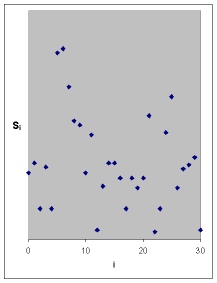
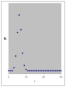
instead of eq. (10). For two filtered channels the exact value of the remaining portion is (m / N) [1 - (2m - h) / N]. For more channels the parameters of the autocorrelation functions of higher order should also be considered for the exact calculation of loss in intensity. For more channels one must consider that by increasing the number of the zero weights, the information matrix M can become singular. To avoid this, the duty cycle c should be decreased. The optimization is not too difficult by computer trials and it can also be performed analytically for fixed models [e.g. for spectrums following eq. (7)]. The use of a smaller duty cycle does not mean any disadvantage for the reason that filtering is effective only for low background, and in these cases a smaller than 1/2 duty cycle can be optimal⁶⁾ . If c is small, the posterior filtration outlined here does not erase too many Z_k, so it can be extended to more channels without making the system underdetermined.

3. Dropped-out points

The posterior filtration can be applied for the appearance of dropped-out points, too. Because of electronic error some Z_k can become false (e.g. contents of some time-channels are erased). These channels can be filtered by the weights w_k = 0, if Z_k is dropped out. Here the decorrelation (3) is of no use. This is shown by computer-simulated measurements. We produced a TOF spectrum by eq. (2), adding Poisson-distributed errors to the Z_k 's. The parameters of the used PRBS: N = 31, m = 6, c = 1/6. The model function: S_i = A exp[- (i - M)² / D²] with A = 100, M = 6, D² = 3 and with background b = 100. Half of the measured points Z_k   were simulated as rejected points. These randomly chosen channels got the mean content Z . (One could not do better.) The spectrum {S_i } was reconstructed by eq. (3), the traditional decorrelation (Fig. 1), and by my method according to eq. (9) (Fig. 2). 

Fig. 1. The spectrum reconstructed with decorrelation (3) is absolutely useless.	Fig. 2. The spectrum reconstructed with direct fitting (9) and with posterior filtration of the dropped-out points show the peak accurately.

The former resulted in an unevaluable spectrum. The latter yields nearly the exact parameters. The mean square deviations of the parameters are about √2 time the MSDs given by the simulation without dropped-out points, but still they are sufficiently small (table 1). It means that the proposed evaluation of experiments with lost counts provides a good result that reflects the loss in accuracy proportionally to the loss of information. As opposed, the formerly used method results in total loss of accuracy due to some loss of information.

Table 1. Estimation for the parameters of TOF spectrum, with posterior filtration of the dropped-out points. In the simulation 50% of the measured points were dropped out.  A is the amplitude, M is the abscissa, D² is the square width of the peak, b is the background level.

4. Summary

A new method is introduced for filtering posterior the correlation TOF spectrum. It has the following advantages over the usual decorrelation technique:

1. The loss of intensity is significantly less.
2. It is no use to add another chopper and gating electronics to the usual TOF correlation arrangement.
3. Filtering is performed after the measurement, so it is adjustable, the channels to be filtered can be chosen a posteriori, and the unfiltered spectrum can also be reconstructed.
4. It fits well to the data evaluation process, yielding the best estimation for the parameters of the spectrum.
5. The dropped-out points can also be filtered by this technique contrary to the usual decorrelation method.

References

1. L. Pal, N. Kroo, P. Pellionisz, F. Szlavik and I. Vizi, Symp. on Neutron inelastic scattering, Copenhagen, (IAEA, Vienna, 1968) vol. 2, p. 407.
2. F. Gompf, W. Reichardt, W. Glaser and K. Beckurts, ibid: p. 417.
3. G. Wilchelmi and F. Gompf, Nucl. Instr. and Meth. 81 (1970) 36.
4. K. Weise, Nucl. Instr. and Meth. 98 (1972) 119.
5. F. Hossfeld, R. Amadori and R. Scherm, Proc. Symp. on Instrumentation of neutron inelastic scattering (IAEA, Vienna, 1970) p. 117.
6. R. von Jan and R. Scherm, Nucl. Instr. and Meth. 80 (1970) 69.
7. R. Amadori and F. Hossfeld, Symp. on Neutron inelastic scattering, Grenoble, IAEA/SM-155/F-5 (1972).
8. F. Hossfeld and R. Amadori, Berichte der Kernforschunganlage Julich (1972).
9. P. Pellionisz, N. Kroo and F. Mezei, Symp. on Neutron inelastic scattering, Grenoble, IAEA/SM-155/F-8 (1972).
10. R. Amadori and F. Hossfeld, Nucl. Instr. and Meth. 124 (1975) 429.
11. R. Amadori, Berichte der Kernforschungsanlage Julich, 1050-FF (1974).
12. L. Cser and L. J. Naszodi, following article.

Back to top

Vol. 161 pp. 163-165 Consideration of the Real Modulation in Correlation Technique Laszlo J. Naszodi Institute of Isotopes of the Hungarian Academy of Sciences

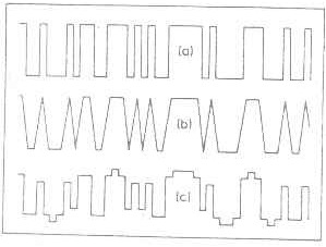
Abstract: The consideration of real modulation requires to replace the equations' system of the correlation TOF technique. The solution and the loss of information coming from the non-ideality are discussed.

In the correlation time-of-flight technique ^1-6) the continuous function T(t) describing the transmission (modulation) is generally represented by an idealized sequence {a_j} of N elements. a_j = 1 if the chopper is open and a_j = 0 if the chopper is closed in the interval jΘ ≤ t < (j+1)Θ (j=0,1,2,...,N-1). Here Θ is the elementary period of the modulation. The matrix equation for the spectrum {S_i} (i=0,1,2,...,N-1) and the measured counts {Z_k} (k=0,1,2,...,N-1) is

Z = AS + b(1)

Where

Z is the vector of the counts;

A is an NxN circular matrix composed from {a_j}, its elements a_ki = a_{k-i mod N} (k,i=0,1,2,...,N-1);

S is the vector of the conventional spectrum elements to be determined;

b is the vector of the background counts assumed to be known and equal in every channel, i.e., b_k = b (k=0,1,2,...,N-1).

The solution of eq. (1) is generally

S = A^-1(Z - b).(2)

Using a pseudo-random binary sequence (PRBS) for chopping, the solution is more simple, since the inversion of A is its transposition, regardless of a multiplying factor and an additive constant:

S = [m(1-c)] ^-1 (A^T - C) Z - b/m,(3)

where m =Σ a_j , the number of open elements in the PRBS;

c = (m-1)/(N-1), the duty cycle of the PRBS;

C is an NxN matrix, full with c.

The i th element of eq. (3) is composed by the cross-correlation between { a_k-i} and {Z_k} and that is why this technique is called correlation technique. Nevertheless, correlation comes about as an inversion in this special case.

The expressions (1), (2) and (3) would be exact only if the pseudo-random modulating function T(t) were rectangular (Fig. 1a), i.e. when the rise and fall time were infinitely short. The physically producible modulations^2-4) do not meet this criterion. The most wide-spread modulation applies a rotating disk that has transparent and blocking sections in accordance with the PRBS. This type of chopper yields a modulating function of triangular or trapezoidal shape (Fig. 1b). It can also be represented by a rectangular sequence of N elements, but the jth element a_j must be equal to the average of the transmission over the jth period, rather than 0 or 1 (Fig. 1c):

ā_j = 1/Θ ∫_jΘ ^(j+1)Θ  T(t) dt          (j=0,1,2,...,N-1)(4)

Fig. 1. The beginning of a modulating function used in Dubna. (a) ideal; (b) real; (c) rectangular representation of the real modulation {aj}.	Fig. 2. The inverse sequence { rj } of { āj } (drawn in reverse order for easier comparison with Fig. 1 a and c).

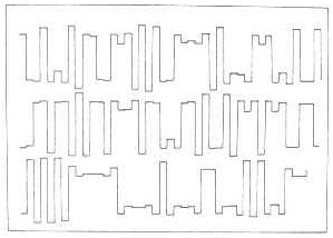
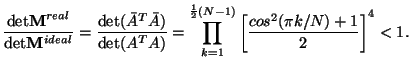
(4) can be expressed simply by linear combination of some elements a_j. For example, if the elementary slits of the chopper are congruent with the diaphragm slit, then

ā_j = (a_j-1 ± 6a_j+a_j+1)/8,(5)

(Fig. 1c). If the incident intensity does not change rapidly inside the jth period, the outcoming intensity is ā _j times the incident intensity and we have to write in eqs. (1) and (2) a circular matrix Ā instead of A, with the elements Ā _ki = ā_k-i(modN). Nevertheless, in eq. (3) the matrix A^T should not be substituted by Ā^T, because for real modulation the S_i is not proportional to the cross-correlation of {ā _k-i} and {Z_k}. (In other words, the inversion of Ā is not proportional to its transposition anymore.) The solution is similar to the general form of (2):

S = R (Z-b), where

R =  Ā^-1 ≠ [m(1-c)] ^-1 (A^T - C)(6)

So, the elements r_j of the circular matrix R are to be determined first to obtain S.

Pelizzari and Postol published a method for obtaining the new decorrelating (inverse) sequence {r_j} empirically⁷⁾: If one takes a well-known spectrum S, its correlation measurement Z (and the known background), then eq. (6) can be regarded as the system of equations for { r_j }. After solving this system they used the obtained inverse sequence for evaluating other measurements. They found that the fluctuations of {S_i} decreased relatively to those obtained by the inversion of the ideal sequence. In principle, this method corrects other systematic imperfections of the chopper, e.g. the unequal transmissions of the open elements, too. Nevertheless, the system (6) is ill conditioned for { r_j }, i.e. the result will be highly erroneous even in the case of small errors of S and of Z.

The inverse sequence can be determined analytically, free from measured errors, too, if the real modulation deviates from ideal primarily because of the finite fall and rise times. One can show⁸⁾ that the circular matrix of the elements (5) can be diagonalized in the form

Ā = UΛU*,(7)

where U is a unitary matrix with the elements of

U_jk = ω^k_j /√N,j, k = 0, 1, ..., N-1;

U* is the transposed conjugate of U;

ω_j = exp (i2πj/N);

Λ is the diagonal matrix of the eigenvalues λ_k of Ā;

λ_k = Σ ā_s ω^s_k      k = 0, 1, ..., N-1;

The inversion of Ā:

R = UΛ^-1U*,(8)

with the elements

R_pq = 1/N  Σ exp[i2π(p-q)k/N]/λ_k = r_{p-q mod N}   p, q = 0, 1, ..., N-1,(9)

i.e. R is the circular matrix of the elements

r_j = 1/N  Σ_k {exp[i2πjk/N] / Σ_s ā_s exp[i2πks /N]},   j = 0, 1, ..., N-1(10)

of the new inverse sequence. If ā_j = a_j, we get back the ideal case: r_j ~ a_-j.

The above computation has been performed for the modulating sequence of the ANL chopper and the result is similar to the decorrelating sequence published in reference 7. One can show that some significant differences come from the statistical errors of the empirical method. Fig. 2 shows the analytically determined inverse sequence of a chopper working at the IBR-30 reactor in Dubna.

The elements differ from the ideal rectangular ones by about 15%. This deviation causes a loss of information, which can be measured by the ratio of the determinants of the information matrices M coming from the ideal and the real modulations. The square root of this ratio is equal to the ratio of the volumes of the dispersion ellipsoids of S obtained from the two modulations¹⁰⁾. In the approximation used in ref. 10 this ratio is ⁹⁾

(11)

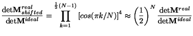
I have to emphasize that this loss arises from the very fact of the non-ideal modulation and not from its consideration. However, if we disregard the real modulation, we disregard the real dispersion ellipsoid and the errors of the S_i's computed in the usual way will be false.

If the time division is shifted by ½ θ, i.e. the channel is centered not at the moment of covering the diaphragm by the slit, then, instead of eq. (5), ā_j = ½ (a_j + a_j+1) or

a _j   = ½ (a_j-1 + a_j), and a similar derivation leads to the expression

(12)

i.e., a half-channel shift of time causes not only a corrigible shift in the spectrum {S_i}, as is the case with an integer-channel shift, but a greater loss in a mathematical statistical sense.

The substitution of the old decorrelating sequence by {r_j } does not change the computation of S significantly and does not increase its time if the sequence used earlier was stored as a set of arithmetic zeros and ones and not of logic constants.

References

1. L. Pal, N. Kroo, P. Pellionisz, F. Szlavik and I. Vizi, Proc. Symp. on Neutron inelastic scattering, Copenhagen (IAEA, Vienna, 1968) vol. 2, p. 407.
2. F. Gompf, W. Reichardt, W. Glaser and K. Beckurts, ibid, p. 417.
3. F. Hossfeld, R. Amadori and R. Scherm, Proc. Symp. on Neutron inelastic scattering, (IAEA, Vienna, 1970) p. 117.
4. J. Gordon, N. Kroo, G. Orban, L. Pal, P.Pellionisz and I. Vizi, Phys. Lett. 26A (1968) 122.
5. N. Kroo and L. Cser, Fizika Elementarnych Tsjastii I Atomnogo Jadra, 8 (1977) 1412 (in Russian).
6. R. Amadori and F. Hossfeld, Proc. Symp. on Neutron inelastic scattering, Grenoble, IAEA/SM-155/F-5 (1972).
7. C. A. Pelizzari and T. A. Postol, Nucl. Instr. and Meth. 143 (1977) 139.
8. P. Rozsa, Linear algebra and its applications (Technical Publisher, Budapest, 1974) p. 254 (in Hungarian).
9. Ibid., p. 267.
10. L. Cser and L. J. Naszodi, Nucl. Instr. and Meth., this issue, p. 141.

Back to top

Vol. 161 pp. 141-145 Estimation for the Parameters of the TOF Spectrum and Measures for the Gain of Correlation Method Laszlo Cser and Laszlo J. Naszodi Joint Institute for Nuclear Research, Dubna, U.S.S.R.

Abstract: A straightforward method is introduced for the data evaluation of correlation measurements. Its advantages over the usual two-step procedure (decorrelation and fitting) are discussed. With the help of the obtained variance-covariance matrix new measures are proposed for the gain of the correlation time-of-flight method compared to the conventional one. These measures are related to the relative accuracy of the final estimated parameters of the spectrum. The optimization of parameters of the chopping sequence is also discussed. Since the problem involves calculations of determinants of large matrices, a new analytical solution is provided which eliminates time consuming computations.  

Back to top

Abstract: Attention is drawn to a bias occuring in the course of calibration. Since the usual assumption of normality leads to an estimate without expected value, here a class of distribution is introduced which does not cause such a deficiency. Even in this class, the correction of the regression line defined with the help of standards might be necessary before estimating the abscissa value belonging to an unknown object. The estimate introduced is compared to the classical and inverse estimates. A mode of eliminating the error by experimental design is also discussed. The calibration process was simulated by computer.

This is my most cited publication. For example, in Journal of Quality Technology Volume 34 · Issue 1 · January 2002 (http://www.asq.org/pub/jqt/past/vol34_issue1/qtec-71.html) Edna Schechtman, Beer Sheva, and Cliff Spiegelman wrote:

"Naszodi (1978) derived a new estimator which is approximately (asymptotically) unbiased, more efficient than the classical estimator, and consistent."

Another citation by James J. McKeon and Raj S. Chhikara, in LINEAR REGRESSION ESTIMATORS IN SAMPLE SURVEYS UNDER CALIBRATION p. 286:

"... the classical estimator has infinite variance. This serious defect can be removed by using a modified classical estimator proposed by Naszodi (1978).
... a modified estimator of X is obtained by X = x - (Y - y)/b(1 + q). This estimator has finite variance and is unbiased to 0(1/n)."

More citation by Christine Osborne, in Statistical Calibration: A Review International Statistical Review Vol. 59, No 3. (December 1991) pp. 309-336

More articles on the topic

Other topics

Articles on Web Design and Development

Articles on Property Appraisal