Thou shalt not pay more property taxes than what thou deserve ...

Articles on Real Property Appraisal

• Introduction to Regression Analysis for Real Property Appraisers
• Common Mistakes in the Application of MRA to Mass Appraisal
• IAAO Mass Appraisal Contest

Appraisers' Workshop, Grand Junction, Co 1997 Introduction to Regression Analysis for Real Property Appraisers Laszlo J. Naszodi Assessment Statistician, Ph.D.

Introduction to the introduction

Our primary source of information is the set of sales data. Sales prices are the indicators of market values. However, not all properties have been sold and most sales did not occur on the appraisal date. We need a mathematical model that guides us how to calculate the value of properties with known characteristics. From the known sales prices and inventory of the sold properties we want to project the values of sold or unsold properties to the appraisal date. Regression analysis is a mean to find the curves and surfaces of the projection. The result of the analysis is a multivariate function that describes the relationship between the value and the characteristics of the property:

In the course of analysis, the characteristics, like square footage, number of bathrooms, location, are known and the parameters, like unit values and neighborhood factors, are unknown. Values are replaced with known prices and the form of the relationship is the question. Note that the task here is turned inside out: not the property value but the parameters are to be determined. Once we figure out the nature described by a function, we can solve our original problem. After the regression analysis we can calculate the value of any property by plugging the found parameters and the characteristics of the property in expression (1). The most common way to display sales prices is two-dimensional graphs. As examples, we can present prices depending on the date of sale or on the heated area: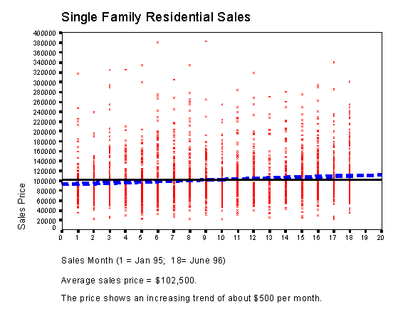

Figure 1.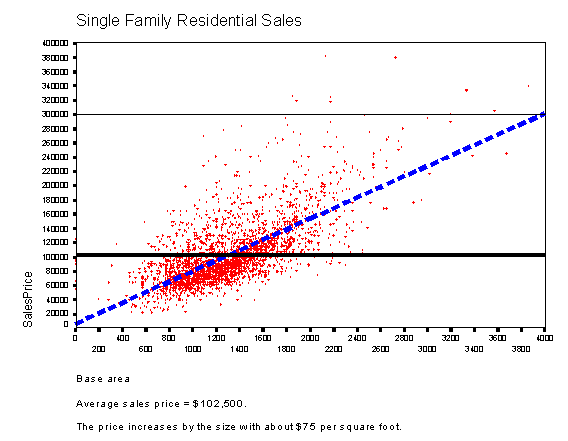

Figure 2.

The above graphs show the relationships between the price and the sales date and between the price and the size of the property. Do they really? What is wrong with these pictures?  What we see is not an established relationship but two clouds and dashed lines laying in the middle of the clouds.

My main goal is to remove the cloud. Mass appraisal should not be a mess of appraisals.  It should be a consistent system of assumptions, proofs of assumptions and application of consequences of the proven assumptions. A model puts the proved assumption in a form of mathematical function.  Our regression analysis aims at finding the function that describes the property value with explainable parameters.

Back to top

IAAO Conference, Chicago, 1995 Common Mistakes in the Application of MRA to Mass Appraisal Laszlo Naszodi Assessment Statistician, Ph.D.

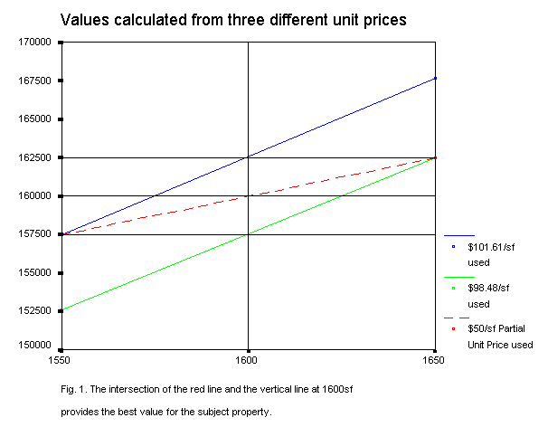
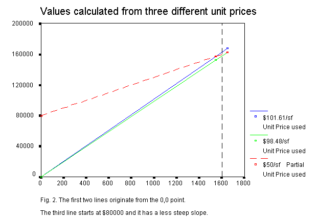
Abstract

In this paper I will attempt to clarify some common mistakes in the appraisal practice.   I will explain why there is no such thing as unit price and why the most logical time trending model is not linear.  In other words, we need to reconsider the basic concepts we operate with.  Through the study of simple cases I will discuss the erroneous notions of using the price-per-square foot approach and standard time trending techniques, some misconceptions that are deeply planted in the appraisal practice. In valuation debates, both appraisers and petitioners hold elementary but unacceptable arguments on the same basis. The proposed alternatives reserve simplicity and solve this controversy. In a third topic I would like to prove that today�s appraisal standards and practices can lead to erroneous inferences, while the exiled MRA can solve the problem.

Back to the basics
If someone hears the expression �flat tax� and does not know anything about the political issues, he or she may think the tax as a constant. In fact, the flat tax promoters mean a function of a constant slope, not of constant value. Further, they attach the idea of deduction and we obtain the most common linear function:

          tax = constant + tax rate * income

or       y = constant + a*x

In case of income tax, the independent variable  x  is the income and the dependent variable  y  is the tax. In the property taxation business, the simplest formula we use is

          value = unit value * units.

To me, a linear function without an additive constant is as questionable as the linear function without a slope.  However, an appraiser may state without risk that the value is equal to $80 times the square footage, while we may ridicule ourselves saying that, regardless of the size, all properties have the value of $100,000.  In a homogeneous neighborhood the latter estimate would work well in 75% of the cases, though.

In the following paper I do not talk about the details of multiple regression analysis. I take it as a known method to determine parameters of model functions that describe the relationship between property value and independent variables.  I will focus on the choice of model functions used in the regression.

Unit price and unit value

This is a real life example. The subject property is a condominium, situated in a high rise building. It has two bathrooms, three bedrooms and an unfinished garage. The heated area is 1600 sqft. The building is new, all sales occurred in the last month of the appraisal period. All comparable properties are on the same front of the building. Three homes of the same features, with same garage size, but with 1650 sqft heated area were sold for $162,500 each. Five comparable homes with 1550 sqft heated area were sold for $157,500 each. What is the value of the subject property?

Calculation using the unit price method

Common sense calculation

The size of heated area of the subject property is between the sizes of the comparable properties, so, its value should be somewhere between the prices of the comparable properties. In the price versus size coordinate system we can connect the two given points of the comparables and read the value of the subject property. It is equal to the value of the linear function at 1600 sqft, i.e., to $160,000. This value is supported by the fact that a 50 sqft  larger property is worth exactly $2,500 more and a 50 sqft smaller property is worth exactly $2,500 less. In other words, the price per square foot in the size range is equal to $50 instead of about $100. The big difference comes from the interpretation of the unit price.

What do we mean on unit price?

As the usual definition, square foot price is the ratio of the price and the square footage. In turn, the value of an unsold property can be calculated by multiplying the square foot price with the square footage. In a price versus size graph, a straight line starting at the zero point illustrates the relationship. This definition implies that a 10% smaller property sells for 10% less and a 10% bigger property sells for 10% more. The slope of the line represents the unit price.

Figure 1 and 2 show the price dependence on the size of heated area. The dashed line connecting the points does not originate from (0,0). However, its slope, about $50/sqft, also represents a type of unit price. If we add (subtract) the product of this unit price and the difference between the sizes of the subject and the comparable properties, we obtain a correct value for the subject property. Let�s call this slope the partial unit price.

Definition: The slope of the price versus units line is called partial unit price.

The method is old, and it is called interpolation. The partial unit price (slope) can be calculated from two arbitrary points of the line. The price difference divided by the unit difference provides the partial unit price:

partial unit price = (price₂ - price₁) / (unit₂ - unit₁) (1)

After rearrangement of formula (1), we obtain a familiar equation:

price₁ =  price ₂ + partial unit price * (unit₁ - unit₂)

or

price of subject = price of comp + partial unit price * (subject units - comp units).(2)

This calculation is not based on the usual unit price approach but on the definition of the partial unit price. Formula (2) is the basic equation of adjustment. If we do not know the price of the subject property, we can estimate its value by adjusting the price of the comparable property:

value_subj =  price_comp + partial unit price * (unit_subj - unit_comp) (3)

Problem 1.1.

Using the figures of the case study, what would be the value of the subject property?

Solution.

From formula (1), the two comparable sales provide

            partial unit price= ($162,500 - $157,500) / (1650 sqft - 1550 sqft) = $50.

Substituting the price and size of any comparable property in formula (3) resolves the conflict and provides the same value:

            value_subj = $162,500 - $50/sqft * (1650 sqft - 1600 sqft) = $160,000 or

            value _subj = $157,500 - $50/sqft * (1550 sqft - 1600 sqft) = $160,000.

Problem 1.2.

Solution:

- The unit price approach presumes that the price versus size line originates from the (0,0) point which is not true.
- The unit price approach is always biased. Depending on the choice of comparable sales, we can produce a higher or a lower value. The interpolation method is consistent and independent of the comparable sale chosen to start the calculation from.
- The partial unit price, gained by linear regression, automatically considers all comparable sales with proper weights.
The simple unit price approach is good for orientation but the final value must be based on a more exact method. A 5 percent error in the unit price creates a 5 percent error in the value. The partial unit price approach is not so sensitive to the errors of the input data.

Conclusion

When we use a concept, we always have to keep in mind, what presumptions are attached to it. Even a frequently used term as unit price can provide misleading values if we misinterpret or neglect its original definition. There is a substantial difference between the usual unit price and the partial unit price. The former corresponds to the primitive unit price approach, the latter to the adjustment approach. Considering that in most cases the price versus size does not originate from the zero point of the coordinate system, we can state that in most cases there is no such thing as unit price. For adjustment and valuation purposes the concept of partial unit price is more adequate. The partial unit price is the slope of the best fitting line on the price versus size graph. It is used in the interpolation to determine the values of unsold properties. The partial unit price is not equal to a (median or average) price divided by a (median or average) size.

Problem 1.3:

Solution

Simple time adjustment

Suppose we have sufficient number of multiple sales during the reappraisal period. Suppose the multiple sales show a solid time trend. Property 1 has been sold in month 0 for $100,000 and in month 6 for 6% more, $106,000. Property 2 has been sold in month 6 for $100,000 and in month 12 for 6% more, $106,000. What would be the time adjusted value of the first property for month 18? $118,000, right? Wrong!

The two pairs of multiple sales show that both in the first six months and in the second six months the relative price increase was a steady 6%. However, it does not mean that the monthly increase was 1% or the annual increase was 12%. If the second property gained 6% from month 6 through month 12, the value of the first property should go up with the same rate in the second and in the third six months. Its value in month 12 is supposed to be $106,000 * 1.06 = $112,360 and it would gain another 6% from month 12 through month 18. Its value in month 18 is supposed to be
$112,360 * 1.06 = $119,102, instead of $118,000.

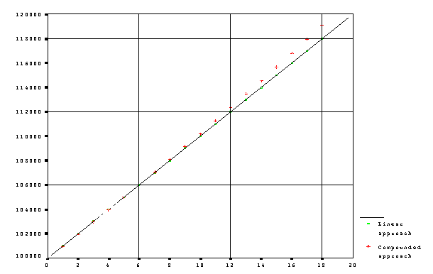
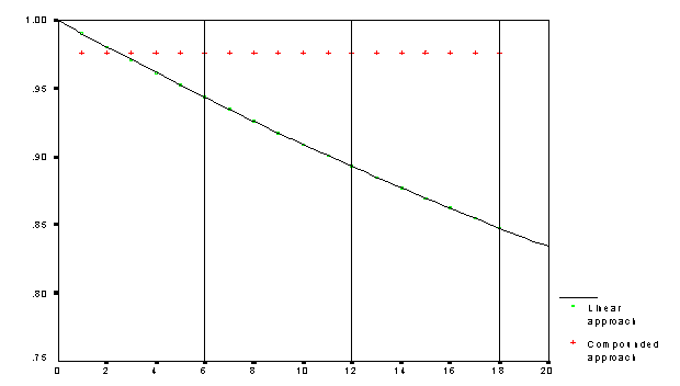
The usual linear approach expects a steady absolute increase per month. Our calculation expected a steady relative increase per month. Let's not fool ourselves! Just because we express the monthly increase in percentage, we may still work with the first method. In our example, a 1% monthly increase of the original value would provide a $118,000 adjusted value, if we used the linear approach and took 118% of the starting value.

In linear approach the rate comes from the equation

value = starting value * (1+rate*month).(4)

The value versus month follows the y = c + a*x function, and equation (4) is linear. However, the relative increase versus month function has a declining shape:

monthly relative increase of value =

(value - previous month value)/previous month value = rate / (1+rate*month)   (5)

where month is the previous month. Formula (4) inherently represents a slowing increase, i.e., the linear approach is nonlinear. If we want to describe a steady market, we should use the compounded approach. The relative monthly change of value should be constant. In other words, the change of every consecutive month is proportional with the value of the previous month:

value - previous month value = rate_{c *} previous month value

which is equivalent to the formula

value = starting value * (1+rate_c)^months.               (6)

Here rate_c stands for the compounded rate. The months versus value graph shows an accelerating change, but in fact, the compounded method represents a constant relative monthly change. Those who have credit cards probably know that, if the interest rate does not change, the increase of the balance accelerates by the time. The way of calculation may be sad but is correct. The bank has not increased the rate, and the amount of balance is what has been increased from month to month.

Do the various approaches make a big difference? Figure 4. shows the graphs of the two approaches. In an 18-month period the lines start at $100,000 and depart about $1000 from each other. A smaller difference may not be significant. As a rule of thumb, we can state: Under 1% monthly increase the two methods do not generate significantly different time adjusted values. If the monthly increase exceeds 1%, the more correct compounded method should be applied.

Fig. 3. Value versus time in linear approach and in compounded approach.
The lower compounded rate provides a higher final value than the higher linear rate.

Problem 2.1.
What would be the monthly rate of increase, based on the above sales data?
Formula (6) can be rewritten as

log (value/starting value) =  months * log(1+rate _c).                              (7)

Replacing the known numbers in (7)

log(1+rate_c) = log(1.06) / 6

rate_c= 0.00976

The monthly compounded rate of increase is 0.976%, less than the 1% rate of the linear approach. However, it provides a higher final value at the end of the period.

Fig. 4. Relative monthly change calculated with linear approach and with compounded approach.
The linear approach is nonlinear. The compounded approach is linear.

Common valuation process versus MRA

An appraiser, valuating real properties by IAAO standards and recommendations, usually follows the steps below:
1a. Determination of time trends from sales. (Univariable regression or other method)
1b. Creation of time adjusted sales prices by projecting prices to the appraisal date.
2a. Determination of parameters describing the dependence of value on inventory items, size, etc.
2b. Determination of predicted values by substituting the actual parameters and inventory data in the value function.
3a. Determination of location dependence. (Univariable sales ratio analysis)
3b. Modification of the model obtained in step 2 with location multiplyers.

The final model is not the result of a multivariable analysis, even if step 2 may utilize MRA. In each step we arbitrarily look at a subspace (projection) of the multidimensional space of the parameter-estimating problem. The obtained parameters are biased, because during the projections we assumed without any basis that they do not correlate. They should not be used as final descriptors of the property value. They would be good initial values of a real multivariable analysis, where all parameters are to be estimated simultaneously without separating some variables and without hijacking the sequence of consideration. The latter practices may result in a set of biased estimates supported by passed significance tests and a series of failed significance tests, although some failed independent variables may show significant influence.

Let me construct a simple but realistic example. A new neighborhood was open for sale. A dozen of properties were sold in a short period of time, all with 1800 square feet heated area, for about $100,000 each. A year later another new neighborhood was open. A dozen sold properties there have houses of only 1600 square feet heated area but their prices also ranged around $100,000. Because all homes and purchases were new, no resales occured during the appraisal period. The common method outlined above would show a zero time rate and a value function independent of location and of size. The result would probably pass all significance tests. In fact, there was a significant price increase by the time and a significant location and/or size dependence.

Questions and answers:

Q: Who are those 'flat tax' maniacs?
A: Some one- or two-dimensional human beings, who can't handle more than one variable at a time.

Q: How do you know a statistician is among normal appraisers?
A: They all try to catch a cat in a dark room, but the statistician yells sometimes: "I got it!"

Q: What is the truth in the appraisal business?
A: There is no cat in the room.

Back to top

IAAO Conference, Chicago, 1995 IAAO Mass Appraisal Contest Laszlo Naszodi Assessment Statistician, Ph.D.

Software and methods used

I have used the SPSS for Windows Base system, version 6.0. For sake of simplicity, I have not utilized any sophisticated elements of the software package. The used features are fundamental and they are available in any other statistical programs. The most complicated analysis I applied was the unweighted linear regression. The nonlinear approaches had been carried out with linear methods.

The model

The mathematical model is basically a multivariate linear function with some multipliers. The effects of most independent variables are described with linear additional members. Some effects, like condition, quality, neighborhood and age are considered with multiplicative factors. However, there is a difference between the usual linear models and that of mine. Instead of the regular linear form

y = b + Σ a _i x _i (1)

I use y -

.

.

.

Similarly, for the description of aging we can choose a factor of linear form

f_eyb = 1+p_eyb (effyr - c_eyb) (8a)

or an exponential one:

f_eyb = exp[A_eyb (effyr - c_eyb)]. (8b)

where  c_eyb can be any given year, as 0, 1900, the present year. Practical considerations prefer a central value of the effective year built. I have used its median, 1979. (See notes in Appendix 2.) Table 1 shows a $962 coefficient for the effective year built, about 1% of the average sale price. By trying the values for p_eyb and A_eyb between 0.009 and 0.02, the exponential model with A_eyb=0.018 turned out to be the best fitting model. The coefficient of EFFY79 also disappeared from the regression. The major difference between the factors feyb and ftime is that the latter should be applied to the land value, too, because the price of the land also depends on the sale date.

7. Determining the neighborhood factor f_nhd.

The neighborhood factor has been determined with the help of regular ratio analysis. If the ratios value / price systematically depart from 1 for a particular neighborhood or economic area, a neighborhood factor is applied to that neighborhood:

f_nhd = 1 / median{value / price}(9)

Advantages of the method

1. 1. The model is not merely a mathematical construction: its parameters have meaningful sense.
2. 2. The first approach, stepwise linear regeression not only provides a usable model but it selects the list of variables that are going to enter in the next approaches.
3. 3. Each step creates an interpretable model. The analyst can stop at any point if he/she feels that the previous step results in a model that sufficiently describes the property value. The improvement can be measured by the changes of simple statistics, as of standard errors and of multiple R square. The first one gives an idea, what range of changes would be significant. The change of the second one report us about the gain of information: what portion of the variability of the values are explained by the last step.
4. 4. Although the model is not constrained by linearity, only linear methods are used for the estimation of non-linear parameters, too.
5. 5. All variables are handled simultaneously. Usual approaches separate the time dependence (univariate time trend analysis), the neighborhood dependence (ratio analysis) and the valuation of the inventory elements (MRA). This separation may cause false results, for example price differences are attributed to the differences in sale dates rather than the increasing size of the newer constructions. My method takes care of these hidden covariances, while it does not contain covariance related parameters, though.

Constrains

1. The calculations could not describe the value of the very small and the very large lands and improvements. We could say that mass appraisal does not work in extreme cases, and we have an excuse. The number of available sales does not allow us to refine the model in these aspects.

More articles on the topic

Other topics

Articles on Web Design and Development

Articles on Correlation and Calibration